Introduction

The Normal Distribution is a continuous probability distribution of a random variable. Anything that we measure with an in-built degree of randomness follows a probability distribution. That means certain values of the measurements of that variable are either more likely or less likely than others. For example, if we decide to measure our own systolic blood pressure, we will find that it does not stay constant at 120 (mm of Hg) as we might think. In fact, our blood pressure will fluctuate throughout the day based on the diurnal rhythms of the body and the stressors that affect us. In fact, the standard deviation of the systolic blood pressure is around 11. So it is completely natural to have a blood pressure of 130 while we are busy at work and then see it drop to 110 after a relaxing bath. However, on average it will hover around 120. If we record this variation and tabulate it, we will see a pattern. There would be a clustering of values around 120 with scattered values around it. As we keep repeating the process, a pattern will emerge. We demonstrate that with an example in the following section.

From discrete to continuous

Let us start by performing a hypothetical experiment where we sample our own blood pressure at regular intervals several times during the waking hours of the day. Let us say we performed 10 measurements. The data might look something like this,

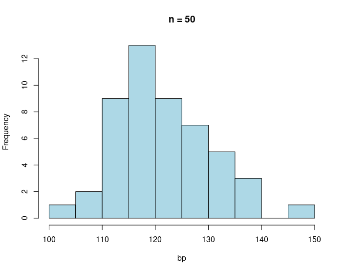
If we sampled few more times

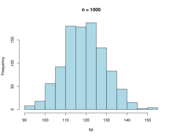
When we increase our sample size to a 1000 data points it starts to look like a bell shaped distribution.

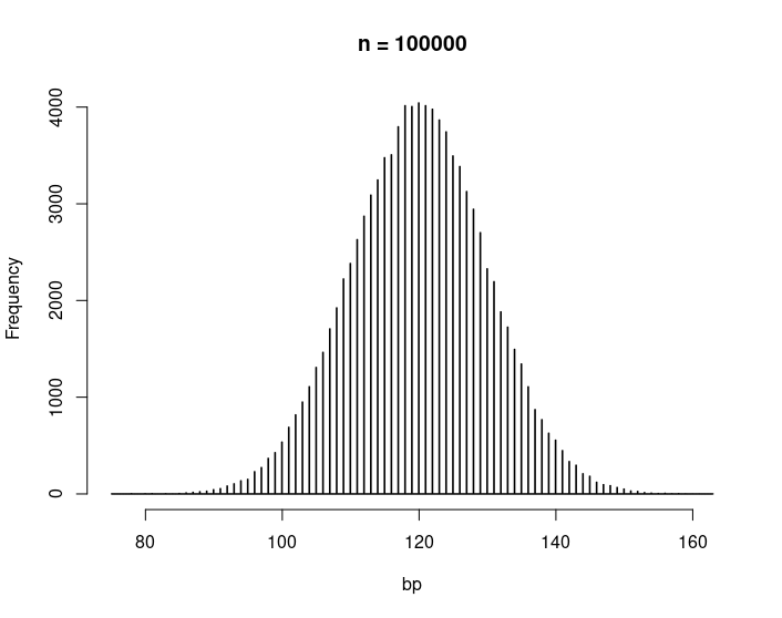
And finally, when we have large quantity of data, the distribution becomes almost continuous.

# above plots can be generated using
> bp = round(rnorm(10, mean = 120, sd = 10))
> hist(bp, breaks = 5, main="n = 10", col="lightblue")
> bp = round(rnorm(50, mean = 120, sd = 10))
> hist(bp, main="n=50", col="lightblue")
> bp = round(rnorm(1000, mean = 120, sd = 10))
> hist(bp, main="n = 1000", col="lightblue")
> bp = round(rnorm(100000, mean = 120, sd = 10))
> hist(bp, breaks=1000, main="n = 100000", col="lightblue")

This bell shaped graph is the Normal Distribution. It is completely specified by only two point estimates of a distribution, mean (\(\mu\) read mu) and variance (\(\sigma^2\) read sigma squared) or equivalently the standard deviation, and is written as: \(N(\mu, \sigma^2)\).

Most data can be modelled using the Normal Distributions but not all. It is the job of the statistician to verify which distribution fits the data best. For example, blood pressure data will follow a normal distribution, but the time interval between arrival of trains at a train station will follow a Poisson distribution. Here, we will only look at simple applications of normal distributions and postpone the discussion of model selection for another lecture.

Probability density function for normal distribution

Normal distribution is uniquely parametrized by the mean and variance. A noemal distribution \(N(\mu, \sigma^2)\) has the probability density function (PDF) \(P(x) = \frac{1}{\sigma \sqrt(2\pi)} exp^{-\frac{1}{2} \left( \frac{x - \mu}{\sigma} \right)^2 }\) Since this is a continuous distribution, the PDF itself has no meaning, only the cumulative distribution function (CDF). We are only interested in the CDF for these lectures.

z-score

z-score of a random event is a measure of how many standard deviations away from the mean is that random event. For example, when someone says that we are witnessing a 6-sigma event, they are saying that we are witnessing a very rare event. Or in other words, that event is so far removed from the average value that the probability of occurrence of that event is almost zero. We can turn this argument around, and claim that if an event occurred due to some intervention and that event is otherwise an improbable event (3-sigma or higher), then the intervention is efficacious. This is utilized in hypothesis testing and finds widespread use among measuring the statistical robustness of well-designed experiments. We will discuss this in the lecture Hypothesis Testing.

Let’s start with an example.
Example 1: The average price of 2-bedroom houses in a small town is \$175,000 with a standard deviation of about $7,000. What is the probability of finding a house for \$165,000 or less (assuming all other parameters like sqft being identical).

Solution: Mean(\(\mu\)) = 175000, SD(\(\sigma\)) = 7000
We find something known as the z-score. The formula for the z-score is
z = \(\frac{X - \mu }{\sigma}\) = (X- mean)/SD
We plug in the values above to get the following z-score,
\(z = \frac{165000-175000}{7000} = -1.42\)
We can then look the corresponding cumulative probability value for the normal distribution table using the R-function.

> z = (165000-175000)/7000
> z
[1] -1.428571
> pnorm(z)
[1] 0.07656373

Therefore, the probability of finding a house listed for $160,000 is 1.6%.

What the z-score does, is that it converts the normal distribution \(N(\mu, \sigma^2)\) to a standard normal distribution \(N(0, 1)\). Therefore, the X-values in the normal distribution are mapped to the z-scores in the standard normal distribution. The advantage is that, we no longer need to painstakingly find the CDF of \(N(\mu, \sigma^2)\). Instead, we just use the CDF for standard normal distribution, which is already calculated to great precision.

Let’s look at few examples on how to calculate the z-scores. Example 2:: If mean = 120, sd = 15, find the z-scores for a. X = 135
b. X = 112
c. X = 101

Solution: For all these problems the mean, and the standard deviation are same: Mean(\(\mu\)) = 120, SD(\(\sigma\)) = 15.
a. X = 135: z = (135-120)/15 = 1
b. X = 112: z = (112-120)/15 = -0.53
c. X = 101: z = (101-120)/15 = -1.27 (rounded from -1.266)
z-scores are usually rounded to 2 decimal places.

Finding the probability using z-score

To find the probability of a random event sampled from a normal distribution, we first find the z-score, and then use that z-score to find the distribution function. Three different scenarios can arise.

1. We want to find the probability of having a value less than a certain X-value.
2. We want to find the probability of having a value greater than a certain X-value.
3. We want to find the probability of having a value between two X-values.

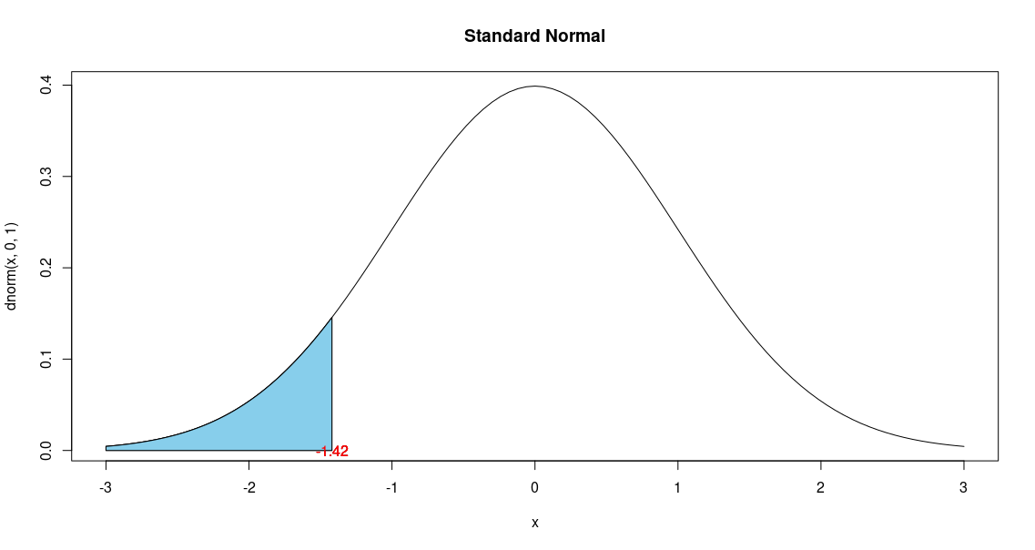
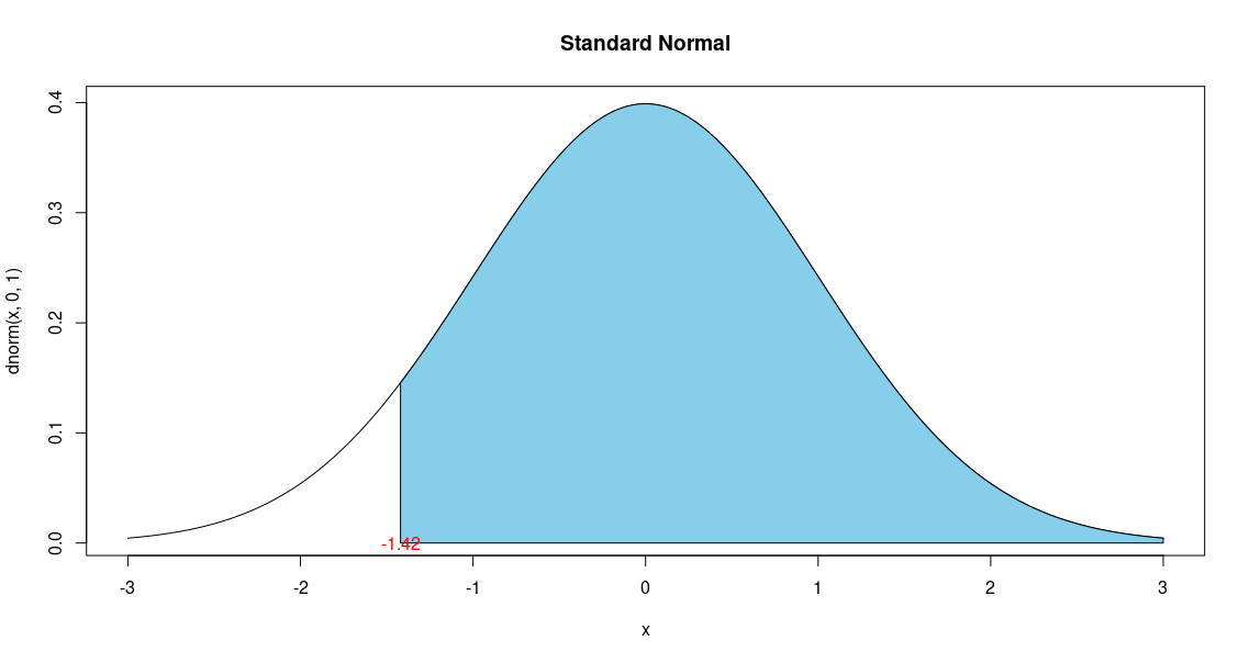
Scenario 1: Find the probability of having a value less than a certain X-value
We have already encountered a problem in this scenario in Example 1 above, where we wanted the probability of a listing less than \$165,000, which is equivalent of asking the area under the PDF to the left of the z-score -1.42.

> curve(dnorm(x,0,1),xlim=c(-3,3),main='Standard Normal') 
> cord.x = c(-3,seq(-3,-1.42,0.01),-1.42) 
> cord.y = c(0, dnorm(seq(-3,-1.42,0.01)), 0)
> polygon(cord.x,cord.y,col='skyblue')
> text(-1.42, 0,'-1.42', col='red')

Scenario 2: Find the probability of having a value greater than a certain X-value
Example 3:: The average price of 2-bedroom houses in a small town is \$175,000 with a standard deviation of about $7,000. What is the probability of finding a house for \$165,000 or more (assuming all other parameters like sqft being identical).

This problem is identical to Example 1 except now we want to see how many houses are selling for more than \$165,000 (rather than less than that value). Everything proceeds identically, until the last step where the probability value has to be subtracted from 1.

Solution: Mean(\(\mu\)) = 175000, SD(\(\sigma\)) = 7000
We plug in the values above to get the following z-score,
\(z = \frac{X - \mu }{\sigma} = \frac{165000-175000}{7000} = -1.42\)

> z = (165000-175000)/7000
> z
[1] -1.428571
> 1-pnorm(z)
[1] 0.9234363

This shows that the probability of finding a house listed for more than \$165,000 is 92.34%. In essence of the pictorial representation, we are essentially finding the area to the right of the graph.

Scenario 3: Find the probability of having a value between two X-values
Example 4:: The average price of 2-bedroom houses in a small town is \$175,000 with a standard deviation of about $7,000. What is the probability of finding houses listed between \$169,000 and \$179,000 (assuming all other parameters like sqft being identical). Solution: Mean(\(\mu\)) = 175000, SD(\(\sigma\)) = 7000
This problem has 2 different z-scores for the 2 different X-values: \(X_1 = 16900, X_2 = 179000\).
\(X_1 = 169000: z = \frac{X - \mu }{\sigma} = \frac{169000-175000}{7000} = -0.86\) \(X_2 = 179000: z = \frac{X - \mu }{\sigma} = \frac{179000-175000}{7000} = 0.57\)

> z1 = (169000-175000)/7000
> z1
[1] -0.8571429
> z2 = (179000-175000)/7000
> z2
[1] 0.5714286
> pnorm(z1)
[1] 0.195683
> pnorm(z2)
[1] 0.7161454
> 0.7161454-0.5204624
[1] 0.195683
> pnorm(z2)-pnorm(z1)
[1] 0.5204624

We have 2 different z-scores; -0.86 and 0.57. We find the corresponding probability density functions for these z-scores, and then we subtract the smaller probability from the larger one (as probabilities have to be greater than 0). The resulting value is the probability of having a listing between \$169,000 and \$179,000 (or a z-score between -0.86 and 0.57). 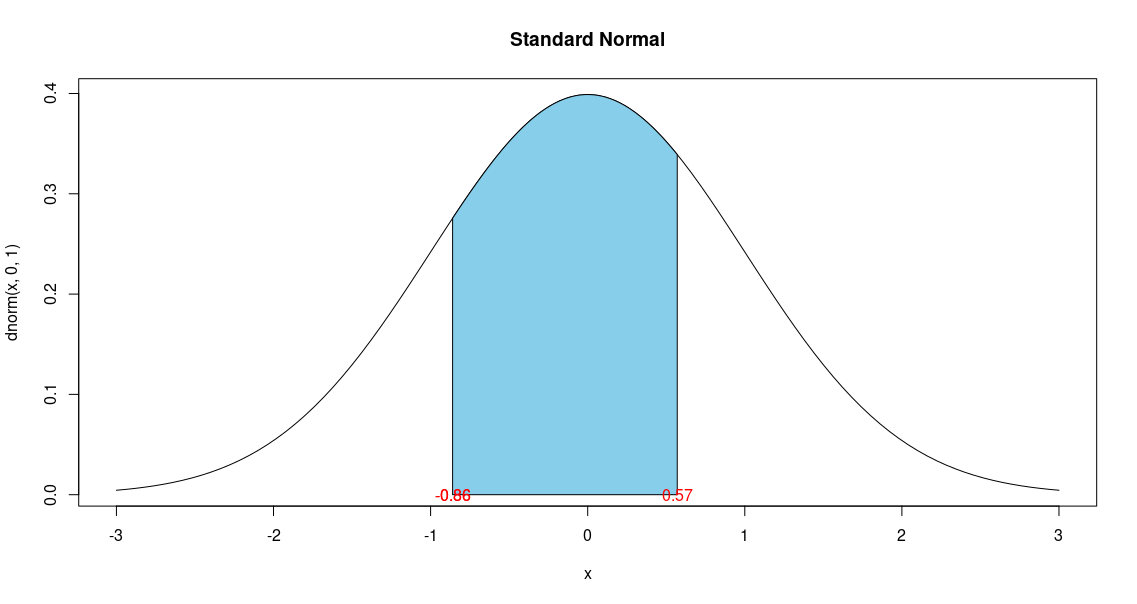There is a 52% chance that a 2-bedroom house will be listed for a price between \$169,000 and \$179,000.

References: Creating shaded areas in R