Introduction
R is a statistical programming language. It has several statistical libraries which facilities fast statistical computations. Python has similar packages (scipy/stats), however, it requires more coding to get the same results in python. Due to the speed of execution, production level code uses Python. For daily research needs R is superior. R is more streamlined and comes with built-in packages to be used a statistical analysis software. We can use R in different ways. We can install it on our computer and use the IDE called R Studio, or we can use cloud computing resources.
Installation
To install R Studio on your computer go to the RStudio website and follow the instructions.
Run R in the cloud
There are several cloud computing options. I will list two.
- Google Colab
Google Colab supports R kernel in addition to python kernels. To launch a Jupyter instance with R kernel go to https://colab.to/r. This is a complete environment and sufficient for all statistical calculations and plotting. The only drawback compared to a local installation is that it does not have all the packages, and it can be difficult to install some uncommon packages with dependencies. - rdrr
This is a website ideal to run snippets of R code. It is not possible to plot using this website (as of writing). It is ideal for one-liners and demonstrations of R code in action. I use this site frequently in my classes. To run R code snippets go to https://rdrr.io/snippets/.
Data types
Data types are the strongest suite for R. Of the possible data types, 3 are of interest to us.
- Vectors
- Matrices
- Data frames
Vectors
Someone told me everything in R is a vector. While that is not entirely correct, it captures the essence of using R. R speeds up statistical calculations by handling long sequences as vectors. Since statistical calculations mostly consists of crunching long sequence of numbers to extract meaning out of them, the ability to load data as a vector is a major productivity boost.
So how do we generate these vectors? We generate a range of integers using the : operator. (If you have not started the R IDE already then do so before proceeding further).
> 0:5
[1] 0 1 2 3 4 5
> 0:10
 [1]  0  1  2  3  4  5  6  7  8  9 10
The first command generates integers from 0 to 5, and the second one generates integers from 0 to 10. To get a vector from this sequence we use
> c(0:5)
[1] 0 1 2 3 4 5
> c(0:10)
 [1]  0  1  2  3  4  5  6  7  8  9 10
c() combines the output into a vector. We will use this to generate vectors.
> c(1:10, 20:30)
 [1]  1  2  3  4  5  6  7  8  9 10 20 21 22 23 24 25 26 27 28 29 30
Combines 2 separate sequences into a single vector.
> p = c(1:10, 20:30)
> p
 [1]  1  2  3  4  5  6  7  8  9 10 20 21 22 23 24 25 26 27 28 29 30
Saves the vector in a variable p which is also called a vector.
We are not restricted to generating integers only. We can generate any sequence using the seq
function.
> seq(0,10,0.25)
 [1]  0.00  0.25  0.50  0.75  1.00  1.25  1.50  1.75  2.00  2.25  2.50  2.75  3.00  3.25
[15]  3.50  3.75  4.00  4.25  4.50  4.75  5.00  5.25  5.50  5.75  6.00  6.25  6.50  6.75
[29]  7.00  7.25  7.50  7.75  8.00  8.25  8.50  8.75  9.00  9.25  9.50  9.75 10.00
Operations on vectors
We can perform mathematical operations on vectors of R in the same way we do with regular vectors.
Multiply each element of a vector by a scalar
> p = c(1:10)*2
> p
 [1]  2  4  6  8 10 12 14 16 18 20
> 2*p
 [1]  4  8 12 16 20 24 28 32 36 40
Add two vectors
> p = c(1:10)
> p
 [1]  1  2  3  4  5  6  7  8  9 10
> q = c(1:10)*2
> q
 [1]  2  4  6  8 10 12 14 16 18 20
> p+q
 [1]  3  6  9 12 15 18 21 24 27 30
Dot product of vectors
> p
 [1]  1  2  3  4  5  6  7  8  9 10
> q
 [1]  2  4  6  8 10 12 14 16 18 20
> p*q
 [1]   2   8  18  32  50  72  98 128 162 200
Slicing
We can extract specific values, or a range of values from vectors or matrices. This is known as slicing.
> p = c(1:5)*2 + c(1:5)^0.5
> p
[1]  3.000000  5.414214  7.732051 10.000000 12.236068
> p[2:4]
[1]  5.414214  7.732051 10.000000
The above code extracts the values in p from location 2 to 4.
Matrices
Matrices can be generated in several ways. Here are some examples.
> matrix(c(1:9))
      [,1]
 [1,]    1
 [2,]    2
 [3,]    3
 [4,]    4
 [5,]    5
 [6,]    6
 [7,]    7
 [8,]    8
 [9,]    9
Passing a vector c(1:9) to the matrix function generates a column matrix when no other
arguments are set.
> matrix(c(0:9), ncol = 2)
     [,1] [,2]
[1,]    0    5
[2,]    1    6
[3,]    2    7
[4,]    3    8
[5,]    4    9
> matrix(c(0:9), nrow = 2)
     [,1] [,2] [,3] [,4] [,5]
[1,]    0    2    4    6    8
[2,]    1    3    5    7    9
Setting values for nrow=2 generates a matrix with 2 rows. If the total number of elements passed
to matrix is not divisible by 2, R will raise an error.
Slicing
Matrices have more one dimension, hence we can slice them in differnt ways.
> p = matrix(c(0:9), nrow = 2)
> p
     [,1] [,2] [,3] [,4] [,5]
[1,]    0    2    4    6    8
[2,]    1    3    5    7    9
> p[1,]
[1] 0 2 4 6 8
This code extracts the first row of the matrix.
> p[2,]
[1] 1 3 5 7 9
The above code extracts the second row of the matrix.
> p[,3]
[1] 4 5
The above code extracts the third column of the matrix.
> p[,3:5]
     [,1] [,2] [,3]
[1,]    4    6    8
[2,]    5    7    9
The above code extracts the columns 3 to 5 from the matrix.
Data frames
Data frames are extremely useful constructs. Imagine an Excel table packaged into a single variable.
Most functions in R, for example lm in linear regression, needs data in data.frame format.
Each column in a data.frame can be of separate type. We will start with datasets formatted
as dataframes that come pre-installed in R. Type in mtcars at the R prompt and hit enter.
> mtcars
                     mpg cyl  disp  hp drat    wt  qsec vs am gear carb
Mazda RX4           21.0   6 160.0 110 3.90 2.620 16.46  0  1    4    4
Mazda RX4 Wag       21.0   6 160.0 110 3.90 2.875 17.02  0  1    4    4
Datsun 710          22.8   4 108.0  93 3.85 2.320 18.61  1  1    4    1
Hornet 4 Drive      21.4   6 258.0 110 3.08 3.215 19.44  1  0    3    1
Hornet Sportabout   18.7   8 360.0 175 3.15 3.440 17.02  0  0    3    2
Valiant             18.1   6 225.0 105 2.76 3.460 20.22  1  0    3    1
Duster 360          14.3   8 360.0 245 3.21 3.570 15.84  0  0    3    4
Merc 240D           24.4   4 146.7  62 3.69 3.190 20.00  1  0    4    2
Merc 230            22.8   4 140.8  95 3.92 3.150 22.90  1  0    4    2
Merc 280            19.2   6 167.6 123 3.92 3.440 18.30  1  0    4    4
Merc 280C           17.8   6 167.6 123 3.92 3.440 18.90  1  0    4    4
Merc 450SE          16.4   8 275.8 180 3.07 4.070 17.40  0  0    3    3
Merc 450SL          17.3   8 275.8 180 3.07 3.730 17.60  0  0    3    3
Merc 450SLC         15.2   8 275.8 180 3.07 3.780 18.00  0  0    3    3
Cadillac Fleetwood  10.4   8 472.0 205 2.93 5.250 17.98  0  0    3    4
Lincoln Continental 10.4   8 460.0 215 3.00 5.424 17.82  0  0    3    4
Chrysler Imperial   14.7   8 440.0 230 3.23 5.345 17.42  0  0    3    4
Fiat 128            32.4   4  78.7  66 4.08 2.200 19.47  1  1    4    1
Honda Civic         30.4   4  75.7  52 4.93 1.615 18.52  1  1    4    2
Toyota Corolla      33.9   4  71.1  65 4.22 1.835 19.90  1  1    4    1
Toyota Corona       21.5   4 120.1  97 3.70 2.465 20.01  1  0    3    1
Dodge Challenger    15.5   8 318.0 150 2.76 3.520 16.87  0  0    3    2
AMC Javelin         15.2   8 304.0 150 3.15 3.435 17.30  0  0    3    2
Camaro Z28          13.3   8 350.0 245 3.73 3.840 15.41  0  0    3    4
Pontiac Firebird    19.2   8 400.0 175 3.08 3.845 17.05  0  0    3    2
Fiat X1-9           27.3   4  79.0  66 4.08 1.935 18.90  1  1    4    1
Porsche 914-2       26.0   4 120.3  91 4.43 2.140 16.70  0  1    5    2
Lotus Europa        30.4   4  95.1 113 3.77 1.513 16.90  1  1    5    2
Ford Pantera L      15.8   8 351.0 264 4.22 3.170 14.50  0  1    5    4
Ferrari Dino        19.7   6 145.0 175 3.62 2.770 15.50  0  1    5    6
Maserati Bora       15.0   8 301.0 335 3.54 3.570 14.60  0  1    5    8
Volvo 142E          21.4   4 121.0 109 4.11 2.780 18.60  1  1    4    2
To explore the basic structure of the data frame without displaying the entire data, we can use
> head(mtcars)
                   mpg cyl disp  hp drat    wt  qsec vs am gear carb
Mazda RX4         21.0   6  160 110 3.90 2.620 16.46  0  1    4    4
Mazda RX4 Wag     21.0   6  160 110 3.90 2.875 17.02  0  1    4    4
Datsun 710        22.8   4  108  93 3.85 2.320 18.61  1  1    4    1
Hornet 4 Drive    21.4   6  258 110 3.08 3.215 19.44  1  0    3    1
Hornet Sportabout 18.7   8  360 175 3.15 3.440 17.02  0  0    3    2
Valiant           18.1   6  225 105 2.76 3.460 20.22  1  0    3    1
We see that the data frame has column names and row names. To grab data from a single column we separate the column name from the dataframe name with a $ symbol.
> mtcars$mpg
 [1] 21.0 21.0 22.8 21.4 18.7 18.1 14.3 24.4 22.8 19.2 17.8 16.4 17.3 15.2 10.4 10.4
[17] 14.7 32.4 30.4 33.9 21.5 15.5 15.2 13.3 19.2 27.3 26.0 30.4 15.8 19.7 15.0 21.4
> mtcars$carb
 [1] 4 4 1 1 2 1 4 2 2 4 4 3 3 3 4 4 4 1 2 1 1 2 2 4 2 1 2 2 4 6 8 2
Statistics with R
There are thousands of statistical packages available to perform statistical computations in R. R itself has several built-in functions to handle the most common statistical computations.
Mean and Standard deviation
> mean(mtcars$mpg)
[1] 20.09062
finds the mean of mpg of cars in the dataset mtcars (see above).
> sd(mtcars$mpg)
[1] 6.026948
finds the standard deviation of mpg of cars in the dataset mtcars (see above).
p-values from z-score
We can calculate the cumulative distribution of a normal distribution using the pnorm() function.
> pnorm(0)
[1] 0.5
> pnorm(-1.96)
[1] 0.0249979
Given a z-score of 1.96 the p-value for a right-tailed test would be
> 1-pnorm(1.96)
[1] 0.0249979
For more insight into how to calculate the p-values, see the tutorial on Normal Distribution.
Plotting with R
Plotting in R is simple when using dataframe.
> head(cars)
  speed dist
1     4    2
2     4   10
3     7    4
4     7   22
5     8   16
6     9   10
> plot(cars)
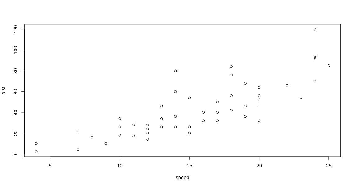 The x and y axes are automatically selected from the columns of the dataframe. Since the
 cars
dataset contain only 2 columns, the first and the second columns are automatically selected as x and
y.
We can generate x and y separately too.
> x=seq(0,10,0.25)
> y = x^2 * exp(-x)
> plot(x,y)
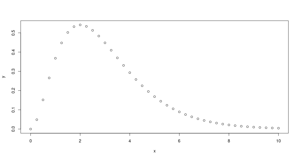 Since x is a vector, the function y(x) is also a vector. The resulting plot with only the data points
is plotted above.
Since x is a vector, the function y(x) is also a vector. The resulting plot with only the data points
is plotted above.
> x=seq(0,10,0.25)
> y = x^2 * exp(-x)
> plot(x,y,type = 'l')
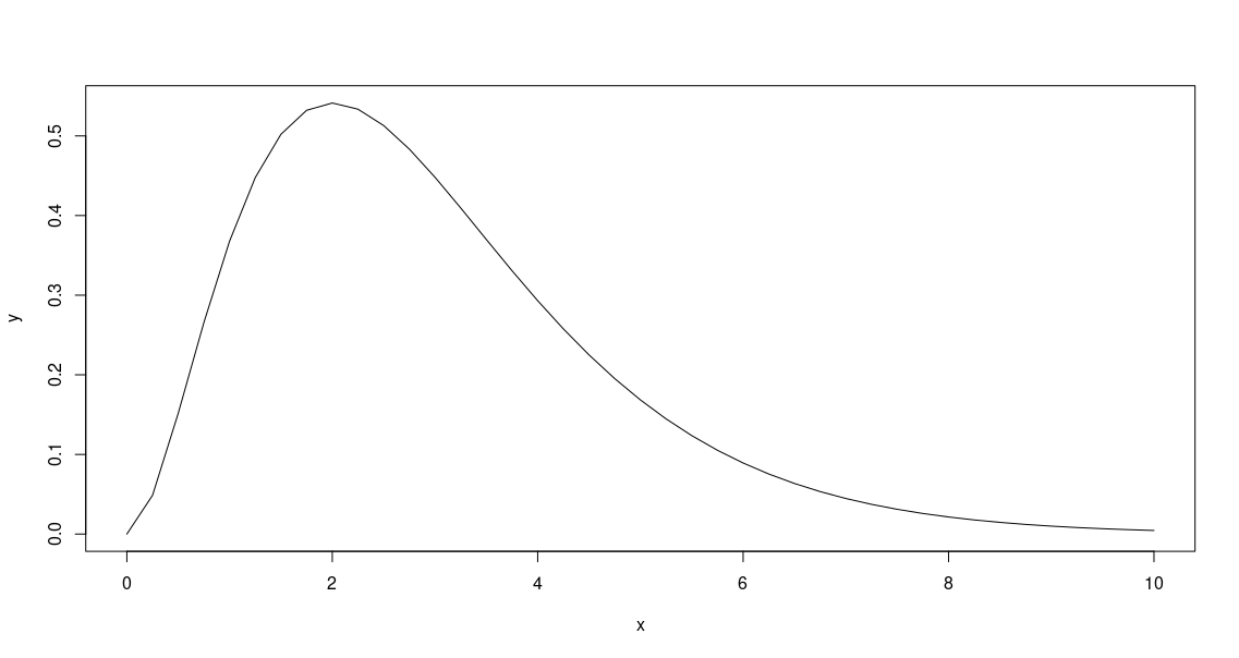 Using
Using type='l' will produce the same plot but with the data points joined by lines.
Plotting histograms
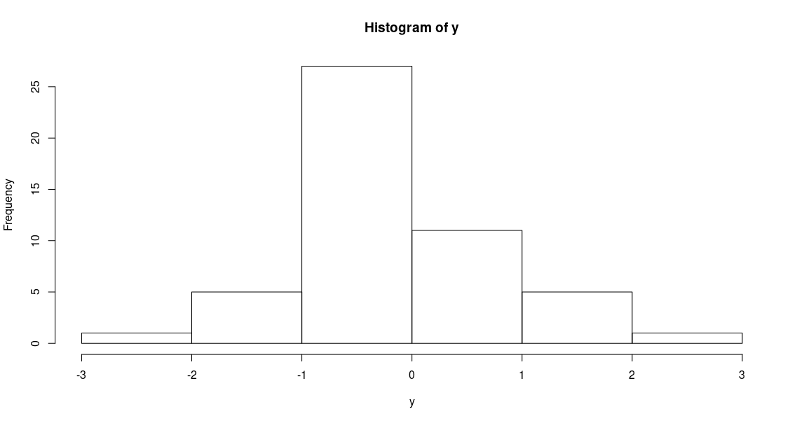
To demonstrate the plotting of histograms we generate 50 random numbers from a normal distribution
> y=rnorm(50)
> hist(y)
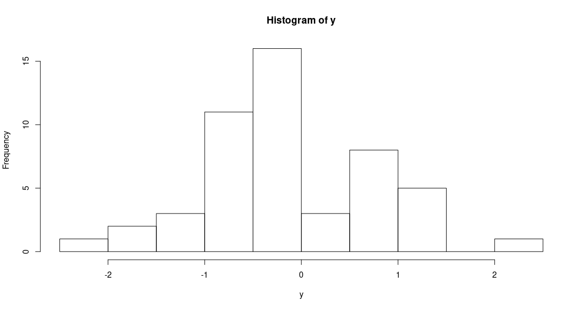
hist() function generates a histogram by automatically choosing a bin size, with the default number of
bins being 10. From the above histogram, it is apparent that the bin size should be increased, to make it
resemble a normal distrobution (from which the values have been sampled). To increase bin size, we can decrease the
number of bins that R uses to plot the histogram by adding the breaks=n argument.
> y=rnorm(50)
> hist(y, breaks=5)