Introduction
Let’s start with a question.
If the covid vaccine has 95% efficacy, then if we sample 100 people,
what is the probability that 95 of them develop immunity?
The answer.
18%
But why 18% and not 95%. This is due to the sampling process. All possible combinations of
(# of immune, # of non-immune) under the constraint that # of immune + # of non-immune = 100
are allowed to occur with a finite probability. Not all those probabilities are equal. Some are
more probable, and some are less probable. Plotting the probabilities produces the following graph.
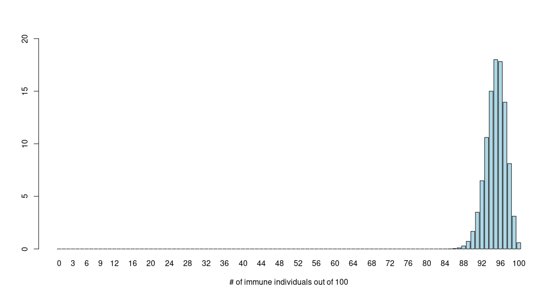
From the plot we see that the probability peaks around 95 and then trails off in either direction. So, although the values sharply peak at 95, the probability of getting 94 immune individuals (out of 100) is similar to that of getting 95 or 96. In fact, a series of values which are not 95 have finite probabilities. The probabilities are distributed over a range of probable values in the form of a bell-shaped structure that we see in the graph. This is known as a distribution, and in this case, it is called a binomial distribution.
Let’s wrap up the discussion about the vaccines. There is no fallacy about the population immunity being 95% and sample immunity being 18%. The probability that exactly 95 out of 100 gets immunity is 18%. What we really want to know is what is the probability that at least 95 out of 100 develops immunity. And that requires a few extra steps. See here for the full discussion.
Binomial Distribution
When we have a binary-valued system i.e. there are only two outcomes, then a collection of events which are subsets of the system, forms a binomial distribution. Consider tossing a coin. There are only two outcomes; heads or tails. {H,T}. Now, if we toss the coin 3 times, then we can get a series of head and tails. The number of heads and tails that we will get at any time would be totally random and determined by the probability of heads from that coin. Let’s say we get {HTH}. This sequence is itself random (the set of all such sequences forms an algebra known as the \(\sigma\)-algebra), but we can calculate its probability.
Let us assume the coin is fair and the probability of landing on heads and tails in equal.
Let
p = P(H) = probability of landing on heads, and
q = P(T) = probability of landing on tails.
The probability of getting HTH is \(P(H) \times P(T) \times P(H) = p \times q \times p = p^2q\).
Now, these are 3 possible ways of getting 2H and 1T since there are three unique possibilities
only {HHT, HTH, THH}. Therefore, the probability of getting 2H and 1T is
\(P(2H,1T) = 3p^2q\)
We can avoid explicit counting of elements, and directly calculate the number of possible events
with 2H and 1T as \({}^3C_2\) since we are choosing 2 heads out of possible 3 outcomes and there
are only \({}^3C_2\) (read 3 choose 2) ways of doing it.
\(P(2H,1T) = {}^3C_2p^2q\)
If we have N tosses, and a series of r Heads, then there must be (N-r) tails.
The probability for {HHHH…(r-times)T….((N-r)-times)} is
\(p \times p \times \cdots (r-times) \times q \times q \times \cdots ((N-r)-times) = p^r q^{N-r}\).
The combined probability for r heads and N-r tails is
\(P(rH,(N-r)T) = {}^NC_r p^r q^{N-r}\)
as there are \({}^NC_r\) (read N choose r) ways of choosing r heads out of N tosses.
This formula is universally applicable to all binomial distributions. Since \(p+q=1\) we can
rewrite this as
\(P(rH,(N-r)T) = {}^NC_r p^r (1-p)^{N-r}\)
Example 1
An unfair coin has a probability of landing on heads 60% of the time. If the same coin is tossed 5 times, what is the probability of getting
- all heads
- 2 heads
- 1 heads
Solution:
1. all heads
Getting all heads when the coin is tossed 5 times means we have 5 heads and 0 tails.
P(H) = p = 60% = 0.6
Since probability of getting tails = P(T) = q = 1 - p (see above)
P(T) = q = 1-0.6 = 0.4
Plugging in the values {N = 5, r = 5, p = 0.6, q = 0.4} in the formula
\(P(rH,(N-r)T) = {}^NC_r p^r (1-p)^{N-r}\)
\(P(5H,0T) = {}^5C_5 \times (0.6)^5 \times (0.4)^0 = 1 \times 0.07776 \times 1 = 0.07776\)
Note: Anything raised to the power of zero is 1. This implies \((0.4)^0 = 1\).
Note: \({}^NC_N = 1\). This implies \({}^5C_5 = 1\).
We convert this to a percentage and round to 2 decimal places and have the final answer
\(P(5H,0T) = 7.78\%\)
Table method Here we show you how to use the table method to calculate the probability of an event belonging to a binomial distribution. Create a table as follows.
| Probability(p) | # of events(r) | p^r | |
|---|---|---|---|
| Success | |||
| Failure | |||
| Total |
Let us arbitrarily label heads as success. We can label tails as success too, and the analysis will remain the same. Here, under the probability column we will write down the individual probabilities of success and failure. In this example, success=heads, so we will write down 0.6 under the probability column in the row for Success, and we will write 0.4 under the probability column in the row for Failure. Remember: We always convert probabilities in percentages to decimals before using them in the formula for the binomial distribution.
| Probability(p) | # of events(r) | \(p^r\) | |
|---|---|---|---|
| Success | 0.6 | ||
| Failure | 0.4 | ||
| Total | 1 |
The total for the first column should always add up to a 1 (100%). Next, we fill the column # of events(r) with the number of success and number of failures. We have 5 heads so there are 5 successes, and there are no tails, so that means there are 0 failures.
| Probability(p) | # of events(r) | \(p^r\) | |
|---|---|---|---|
| Success | 0.6 | 5 | |
| Failure | 0.4 | 0 | |
| Total | 1 | 5 |
The total for the second column should always add up to the toal number of events (5 coin tosses). Now, for the third column we exponentiate the values in column 1 with the values in column 2.
| Probability(p) | # of events(r) | \(p^r\) | |
|---|---|---|---|
| Success | 0.6 | 5 | \((0.6)^5\) |
| Failure | 0.4 | 0 | \((0.4)^0\) |
| Total | 1 | 5 | \({}^5C_5\) |
We did not do a total in the last row of the last column. Instead, we found the pre-factor \({}^NC_r\). If this is confusing you can ignore the last row.
Now, multiply everything in the last column, and you will have your answer.
\(P(5H,0T) = {}^5C_5 \times (0.6)^5 \times (0.4)^0 = 1 \times 0.07776 \times 1 = 0.07776 = 7.78\%\)
Although, this process might seem contrived and a roundabout way of calculating obvious quantities, I have noticed through experience that students perform better with the table method when presented with a complex in binomial distribution (see Example 2 below). Students frequently match the number of successes with probability of failures. The table method provides a visual aid to prevent this mistake.
2. 2 heads
Plugging in the values {N = 5, r = 2, p = 0.6, q = 0.4} in the formula
\(P(rH,(N-r)T) = {}^NC_r p^r (1-p)^{N-r}\)
\(P(2H,3T) = {}^5C_2 \times (0.6)^2 \times (0.4)^{5-2} = 10 \times (0.6)^2 \times (0.4)^3 = 0.2304 = 23.04\%\)
Table method
| Probability(p) | # of events(r) | \(p^r\) | |
|---|---|---|---|
| Success | 0.6 | 2 | \((0.6)^2\) |
| Failure | 0.4 | 3 | \((0.4)^3\) |
| Total | 1 | 5 | \({}^5C_2\) |
3. 1 heads
Plugging in the values {N = 5, r = 1, p = 0.6, q = 0.4} in the formula
\(P(rH,(N-r)T) = {}^NC_r p^r (1-p)^{N-r}\)
\(P(1H,4T) = {}^5C_1 \times (0.6)^1 \times (0.4)^{5-1} = 5 \times (0.6) \times (0.4)^4 = 0.0768 = 7.68\%\)
Table method
| Probability(p) | # of events(r) | \(p^r\) | |
|---|---|---|---|
| Success | 0.6 | 1 | \((0.6)^1\) |
| Failure | 0.4 | 4 | \((0.4)^4\) |
| Total | 1 | 5 | \({}^5C_1\) |
Example 2
If the covid vaccine has 95% efficacy, then if we sample 100 people, what is the probability that 95 of them develop immunity?
Solution:
In this problem there are only two outcomes - developing immunity after the vaccine, and not
developing immunity after the vaccine. Therefore, the outcomes follow the binomial distribution.
Let us label developing immunity as success and not developing immunity as failure.
Then
probability of success = p = 0.95 (probability of developing immunity is 95%).
probability of failure = q = 1 - 0.95 = 0.05 (since p+q=1).
We are assuming 95 out of the 100 people in the sample of 100 develop immunity. Therefore,
Number of success = 95
Number of failure = 5
Table method
| Probability(p) | # of events(r) | \(p^r\) | |
|---|---|---|---|
| Success | 0.95 | 95 | \((0.95)^{95}\) |
| Failure | 0.05 | 5 | \((0.05)^5\) |
| Total | 1 | 5 | \({}^{100}C_{95}\) |
P(95 immune, 5 not immune) = \({}^{100}C_{95} \times (0.95)^{95} \times (0.05)^5 = 0.18 = 18\%\)
R Lab
Now, we will learn howto find the probabilities of a binomial distribution using the R package. Specifically, we will learn three things.
- How to calculate probability of a single event using R
- How to calculate the entire binomial distribution using R
- How to plot your binomial distribution
At the end of this section you should be able to generate the plot at the beginning of this tutorial.
If you are unfamiliar with the R package then read this first: Quick Introduction to R.
Combinations in R
Combinations are computed in R using the function choose().
> choose(5,2)
[1] 10
> choose(5,3)
[1] 10
Calculating probability of a single event from a binomial distribution
Example 1.3 Calculating the probability of P(2H,3T) from Example 1.3 above \(P(2H,3T) = {}^5C_2 \times (0.6)^2 \times (0.4)^{5-2} = 10 \times (0.6)^2 \times (0.4)^3 = 0.2304 = 23.04\%\) using R we get
> choose(5,2)*(0.6)^2*(0.4)^3
[1] 0.2304
Example 2
Calculating the probability of P(95 immune, 5 not immune) from Example 2 above
P(95 immune, 5 not immune) = \({}^{100}C_{95} \times (0.95)^{95} \times (0.05)^5 = 0.18 = 18\%\)
using R we get
> choose(100,95)*(0.95)^95*(0.05)^5
[1] 0.1800178
Calculating probabilities of multiple events from a binomial distribution
Example 1 Here we calculate the probabilities of all possible outcomes of tossing an unfair coin 5 times.
> n=c(0:5)
> n
[1] 0 1 2 3 4 5
> choose(5,n)*(0.6)^n*(0.4)^(5-n)
[1] 0.01024 0.07680 0.23040 0.34560 0.25920 0.07776
We first define a sequence of all possible outcomes for heads (or tails) and save the sequence as a vector,
n=c(0:5). Then, we define the binomial probability distribution function (PDF) on this vector. The function
iterates over each value and calculates the corresponding probability and stores in another vector.
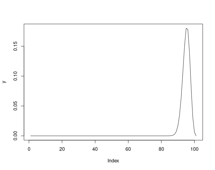
Example 2 The vector of all possible outcomes out of the sample of 100 are all integers from 0 to 100. The binomial PDF is defined on these values.
> n=seq(0:100)
> y=choose(100,n)*(0.95)^n*(0.05)^(100-n)*100
We can plot the probability distribution function as a continuous plot
> plot(y, type ='l')
 However, since this is a discrete distribution we should plot it as a barplot
> n=c(0:100)
> p = choose(100,n)*(0.95)^n*(0.05)^(100-n)*100
> barplot(p, xlab = "# of immune individuals out of 100", ylim=c(0,20), col = "lightblue", names.arg = c(0:100))
The argument ylim=c(0,20) restricts the y-values between 0 and 20 since we do not have any probability values
beyond 20%. names.arg = c(0:100) sets the x labels.